Vision Transformer (二)

Attention

原文地址：https://zhuanlan.zhihu.com/p/342261872

Transformer+Classification：用于分类任务的 Transformer(ICLR2021)¶

论文名称：An Image is Worth 16x16 Words:Transformers for Image Recognition at Scale

论文地址：

https://arxiv.org/abs/2010.11929

5.1 ViT 原理分析：

这个工作本着尽可能少修改的原则，将原版的 Transformer 开箱即用地迁移到分类任务上面。并且作者认为没有必要总是依赖于 CNN，只用 Transformer 也能够在分类任务中表现很好，尤其是在使用大规模训练集的时候。同时，在大规模数据集上预训练好的模型，在迁移到中等数据集或小数据集的分类任务上以后，也能取得比 CNN 更优的性能。下面看具体的方法：

图片预处理：分块和降维

这个工作首先把\(\text{x}\in H\times W\times C\) 的图像，变成一个 \(\text{x}_p\in N\times (P^2\cdot C)\) 的 sequence of flattened 2D patches。它可以看做是一系列的展平的 2D 块的序列，这个序列中一共有 \(N=HW/P^2\) 个展平的 2D 块，每个块的维度是 \((P^2\cdot C)\) 。其中 \(P\) 是块大小， \(C\) 是 channel 数。

注意作者做这步变化的意图： 根据我们之前的讲解 ，Transformer 希望输入一个二维的矩阵 \((N,D)\) ，其中 \(N\) 是 sequence 的长度， \(D\) 是 sequence 的每个向量的维度，常用 256。

所以这里也要设法把 \(H\times W\times C\) 的三维图片转化成 \((N,D)\) 的二维输入。

所以有： \(H\times W\times C\rightarrow N\times (P^2\cdot C),\text{where}\;N=HW/P^2\) 。

其中，\(N\) 是 Transformer 输入的 sequence 的长度。

代码是：

x = rearrange(img, 'b c (h p1) (w p2) -> b (h w) (p1 p2 c)', p1=p, p2=p)

具体是采用了 einops 库实现，具体可以参考这篇博客。

科技猛兽：PyTorch 70.einops：优雅地操作张量维度

现在得到的向量维度是： \(\text{x}_p\in N\times (P^2\cdot C)\) ，要转化成 \((N,D)\) 的二维输入，我们还需要做一步叫做 Patch Embedding 的步骤。

Patch Embedding¶

方法是对每个向量都做一个线性变换（即全连接层），压缩后的维度为 \(D\) ，这里我们称其为 Patch Embedding。

\[\mathbf{z}_0 = [ \color{darkgreen}{\mathbf{x}_\text{class}}; \, \color{crimson }{\mathbf{x}^1_p \mathbf{E}; \, \mathbf{x}^2_p \mathbf{E}; \cdots; \, \mathbf{x}^{N}_p \mathbf{E} }] + \mathbf{E}_{pos} \tag{5.1}\]

这个全连接层就是上式 (5.1) 中的 \(\color{crimson}{\mathbf{E}}\) ，它的输入维度大小是 \((P^2\cdot C)\) ，输出维度大小是 \(D\)。

# 将3072变成dim，假设是1024
self.patch_to_embedding = nn.Linear(patch_dim, dim)
x = self.patch_to_embedding(x)

注意这里的绿色字体 \(\color{darkgreen}{\mathbf{x}_\text{class}}\) ，假设切成 9 个块，但是最终到 Transfomer 输入是 10 个向量，这是人为增加的一个向量。

为什么要追加这个向量？

如果没有这个向量，假设 \(N=9\) 个向量输入 Transformer Encoder，输出 9 个编码向量，然后呢？对于分类任务而言，我应该取哪个输出向量进行后续分类呢？

不知道。干脆就再来一个向量 \(\color{darkgreen}{\mathbf{x}_\text{class}}(\text{vector,dim}=D)\) ，这个向量是可学习的嵌入向量，它和那 9 个向量一并输入 Transfomer Encoder，输出 1+9 个编码向量。然后就用第 0 个编码向量，即 \(\color{darkgreen}{\mathbf{x}_\text{class}}\) 的输出进行分类预测即可。

这么做的原因可以理解为：ViT 其实只用到了 Transformer 的 Encoder，而并没有用到 Decoder，而 \(\color{darkgreen}{\mathbf{x}_\text{class}}\) 的作用有点类似于解码器中的 \(\text{Query}\) 的作用，相对应的 \(\text{Key,Value}\) 就是其他 9 个编码向量的输出。

\(\color{darkgreen}{\mathbf{x}_\text{class}}\) 是一个可学习的嵌入向量，它的意义说通俗一点为：寻找其他 9 个输入向量对应的 \(\text{image}\) 的类别。

代码为：

# dim=1024
self.cls_token = nn.Parameter(torch.randn(1, 1, dim))

# forward前向代码
# 变成(b,64,1024)
cls_tokens = repeat(self.cls_token, '() n d -> b n d', b=b)
# 跟前面的分块进行concat
# 额外追加token，变成b,65,1024
x = torch.cat((cls_tokens, x), dim=1)

Positional Encoding¶

按照 Transformer 的位置编码的习惯，这个工作也使用了位置编码。引入了一个 Positional encoding \(\color{purple}{\mathbf{E}_{pos}}\) 来加入序列的位置信息，同样在这里也引入了 pos_embedding，是用一个可训练的变量。

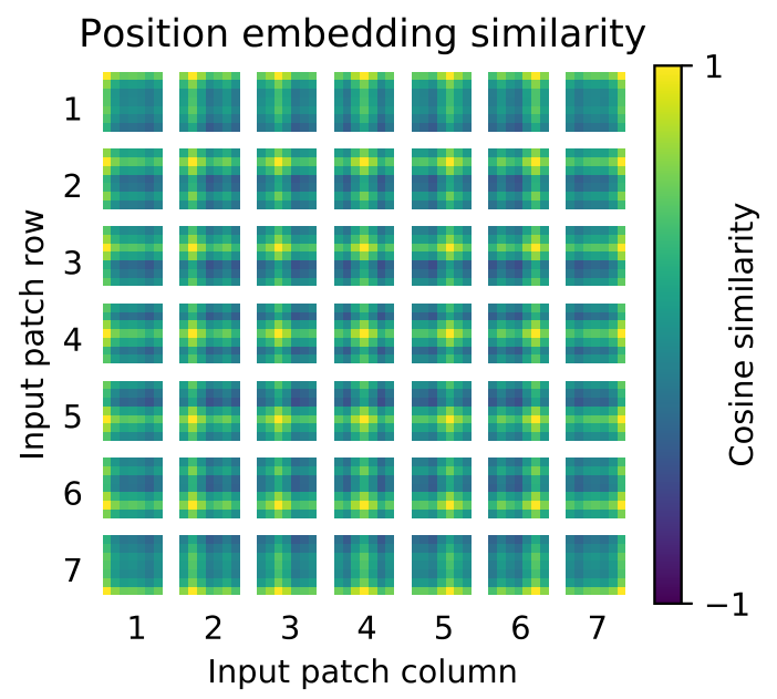
\[\mathbf{z}_0 = [ \mathbf{x}_\text{class}; \, \color{black}{\mathbf{x}^1_p \mathbf{E}; \, \mathbf{x}^2_p \mathbf{E}; \cdots; \, \mathbf{x}^{N}_p \mathbf{E} }] + \color{purple}{\mathbf{E}_{pos}} \tag{5.2}\]

没有采用原版 Transformer 的 \(\text{sincos}\) 编码，而是直接设置为可学习的 Positional Encoding，效果差不多。对训练好的 pos_embedding 进行可视化，如下图所示。我们发现，位置越接近，往往具有更相似的位置编码。此外，出现了行列结构；同一行 / 列中的 patch 具有相似的位置编码。

# num_patches=64，dim=1024,+1是因为多了一个cls开启解码标志
self.pos_embedding = nn.Parameter(torch.randn(1, num_patches + 1, dim))

Transformer Encoder 的前向过程

\[ \begin{aligned} \mathbf{z}_0 & =\left[\mathbf{x}_{\text {class }} ; \mathbf{x}_p^1 \mathbf{E} ; \mathbf{x}_p^2 \mathbf{E} ; \cdots ; \mathbf{x}_p^N \mathbf{E}\right]+\mathbf{E}_{p o s}, & & \mathbf{E} \in \mathbb{R}^{\left(P^2 \cdot C\right) \times D}, \mathbf{E}_{p o s} \in \mathbb{R}^{(N+1) \times D} \\ \mathbf{z}_{\ell}^{\prime} & =\operatorname{MSA}\left(\operatorname{LN}\left(\mathbf{z}_{\ell-1}\right)\right)+\mathbf{z}_{\ell-1}, & & \ell=1 \ldots L \\ \mathbf{z}_{\ell} & =\operatorname{MLP}\left(\operatorname{LN}\left(\mathbf{z}_{\ell}^{\prime}\right)\right)+\mathbf{z}_{\ell}^{\prime}, & & \ell=1 \ldots L \\ \mathbf{y} & =\operatorname{LN}\left(\mathbf{z}_L^0\right) & & \end{aligned} \]

其中，第 1 个式子为上面讲到的 Patch Embedding 和 Positional Encoding 的过程。

第 2 个式子为 Transformer Encoder 的 \(\color{purple}{\text{Multi-head Self-attention, Add and Norm}}\) 的过程，重复 \(L\) 次。

第 3 个式子为 Transformer Encoder 的 \(\color{teal}{\text{Feed Forward Network, Add and Norm}}\) 的过程，重复 \(L\) 次。

作者采用的是没有任何改动的 transformer。

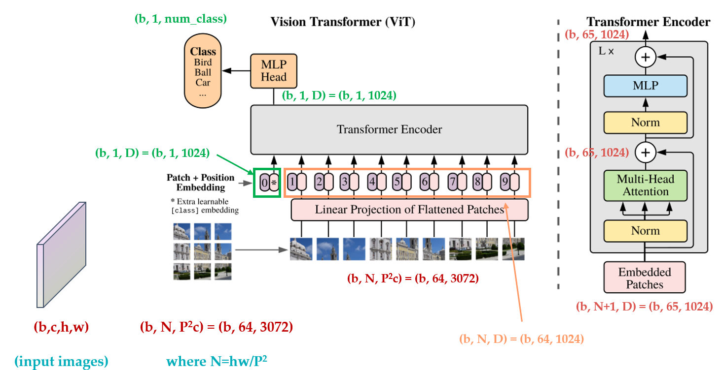
最后是一个 \(\text{MLP}\) 的 \(\text{Classification Head}\) ，整个的结构只有这些，如下图所示，为了方便读者的理解，我把变量的维度变化过程标注在了图中。

训练方法：

先在大数据集上预训练，再迁移到小数据集上面。做法是把 ViT 的 \(\color{purple}{\text{prediction head}}\) 去掉，换成一个 \(D\times K\) 的 \(\color{purple}{\text{Feed Forward Layer}}\) 。其中 \(K\) 为对应数据集的类别数。

当输入的图片是更大的 shape 时，patch size \(P\) 保持不变，则 \(N=HW/P^2\) 会增大。

ViT 可以处理任意 \(N\) 的输入，但是 Positional Encoding 是按照预训练的输入图片的尺寸设计的，所以输入图片变大之后，Positional Encoding 需要根据它们在原始图像中的位置做 2D 插值。

最后，展示下 ViT 的动态过程：

Experiments：

预训练模型使用到的数据集有：

ILSVRC-2012 ImageNet dataset：1000 classes
ImageNet-21k：21k classes
JFT：18k High Resolution Images

将预训练迁移到的数据集有：

CIFAR-10/100
Oxford-IIIT Pets
Oxford Flowers-102
VTAB

作者设计了 3 种不同答小的 ViT 模型，它们分别是：

DModel	Layers	Hidden size	MLP size	Heads	Params
ViT-Base	12	768	3072	12	86M
ViT-Large	24	1024	4096	16	307M
ViT-Huge	32	1280	5120	16	632M

ViT-L/16 代表 ViT-Large + 16 patch size \(P\)

评价指标 \(\text{Metrics}\) ：

结果都是下游数据集上经过 finetune 之后的 Accuracy，记录的是在各自数据集上 finetune 后的性能。

实验 1：性能对比

实验结果如下图所示，整体模型还是挺大的，而经过大数据集的预训练后，性能也超过了当前 CNN 的一些 SOTA 结果。对比的 CNN 模型主要是：

2020 年 ECCV 的 Big Transfer (BiT) 模型，它使用大的 ResNet 进行有监督转移学习。

2020 年 CVPR 的 Noisy Student 模型，这是一个在 ImageNet 和 JFT300M 上使用半监督学习进行训练的大型高效网络，去掉了标签。

All models were trained on TPUv3 hardware。

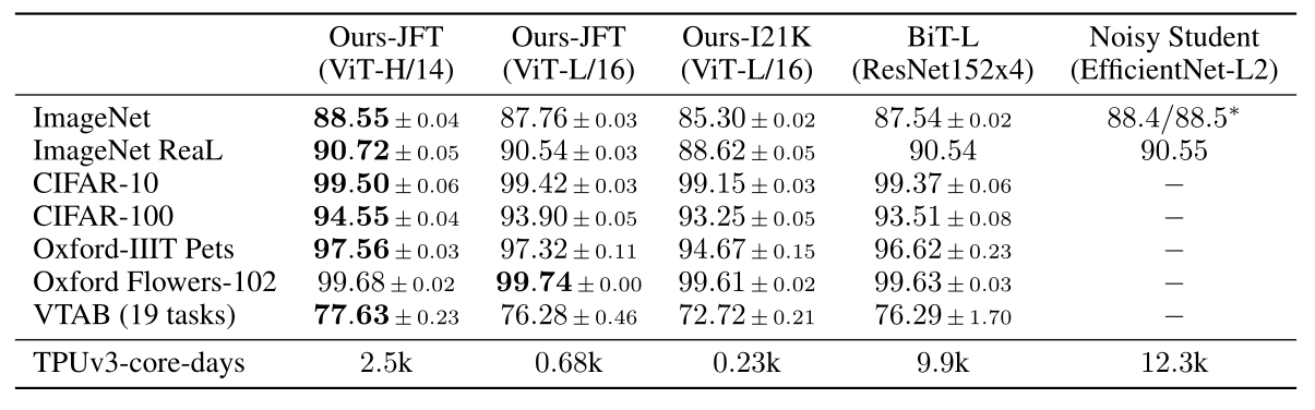
在 JFT-300M 上预先训练的较小的 ViT-L/16 模型在所有任务上都优于 BiT-L(在同一数据集上预先训练的)，同时训练所需的计算资源要少得多。更大的模型 ViT-H/14 进一步提高了性能，特别是在更具挑战性的数据集上——ImageNet, CIFAR-100 和 VTAB 数据集。与现有技术相比，该模型预训练所需的计算量仍然要少得多。

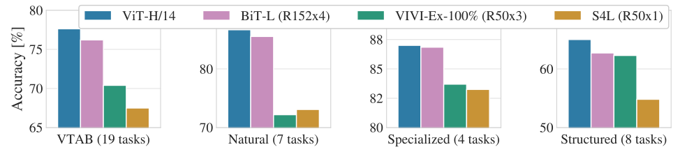
下图为 VTAB 数据集在 Natural, Specialized, 和 Structured 子任务与 CNN 模型相比的性能，ViT 模型仍然可以取得最优。

实验 2：ViT 对预训练数据的要求

ViT 对于预训练数据的规模要求到底有多苛刻？

作者分别在下面这几个数据集上进行预训练：ImageNet, ImageNet-21k, 和 JFT-300M。

结果如下图所示：

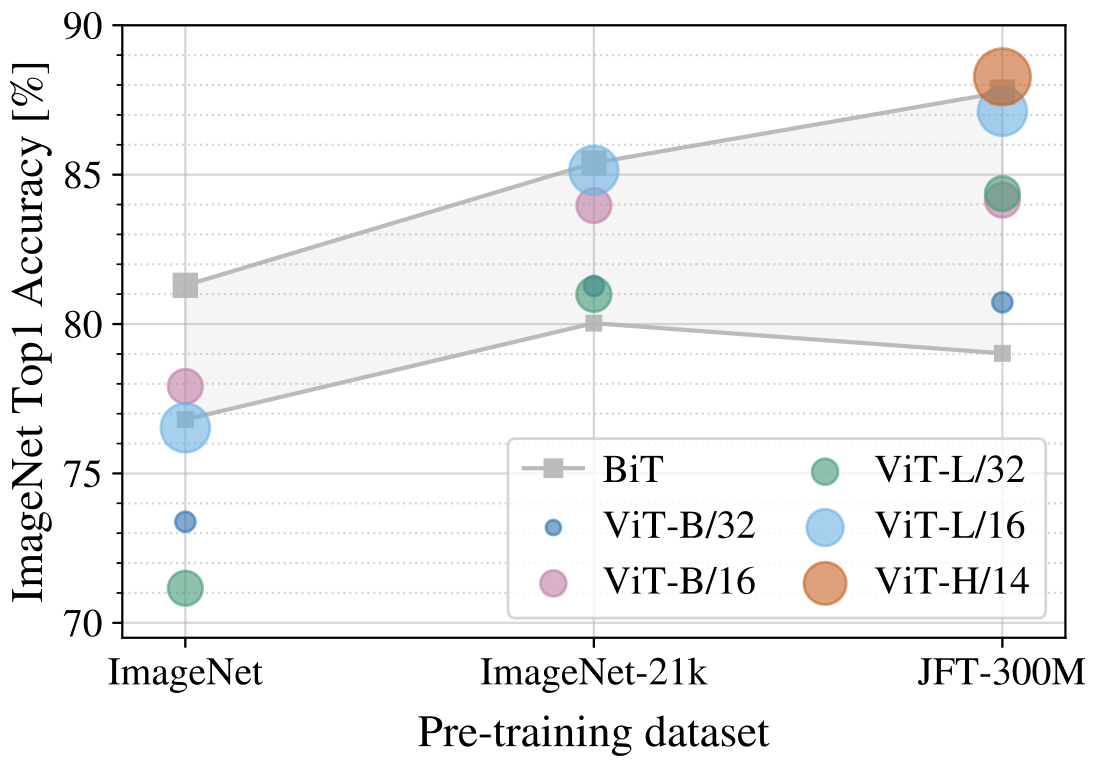
我们发现：当在最小数据集 ImageNet 上进行预训练时，尽管进行了大量的正则化等操作，但 ViT - 大模型的性能不如 ViT-Base 模型。

但是有了稍微大一点的 ImageNet-21k 预训练，它们的表现也差不多。

只有到了 JFT 300M，我们才能看到更大的 ViT 模型全部优势。图 3 还显示了不同大小的 BiT 模型跨越的性能区域。BiT CNNs 在 ImageNet 上的表现优于 ViT(尽管进行了正则化优化)，但在更大的数据集上，ViT 超过了所有的模型，取得了 SOTA。

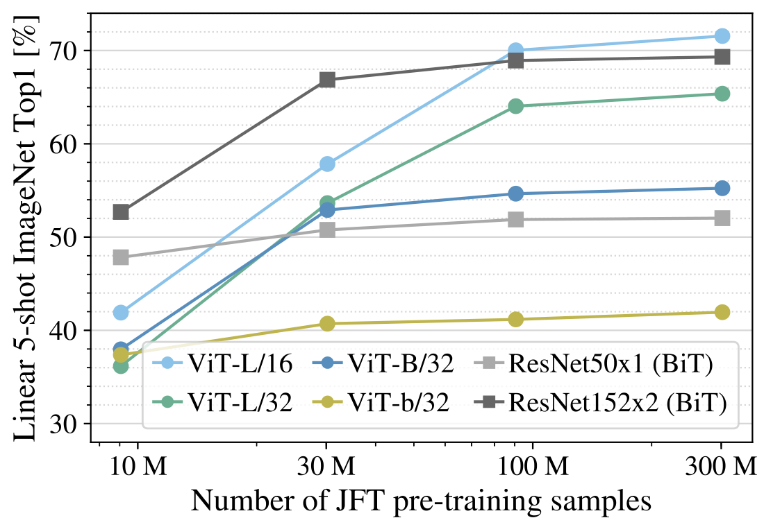
作者还进行了一个实验： 在 9M、30M 和 90M 的随机子集以及完整的 JFT300M 数据集上训练模型，结果如下图所示。 ViT 在较小数据集上的计算成本比 ResNet 高， ViT-B/32 比 ResNet50 稍快；它在 9M 子集上表现更差，但在 90M + 子集上表现更好。ResNet152x2 和 ViT-L/16 也是如此。这个结果强化了一种直觉，即：

残差对于较小的数据集是有用的，但是对于较大的数据集，像 attention 一样学习相关性就足够了，甚至是更好的选择。

实验 3：ViT 的注意力机制 Attention

作者还给了注意力观察得到的图片块， Self-attention 使得 ViT 能够整合整个图像中的信息，甚至是最底层的信息。作者欲探究网络在多大程度上利用了这种能力。

具体来说，我们根据注意力权重计算图像空间中整合信息的平均距离，如下图所示。

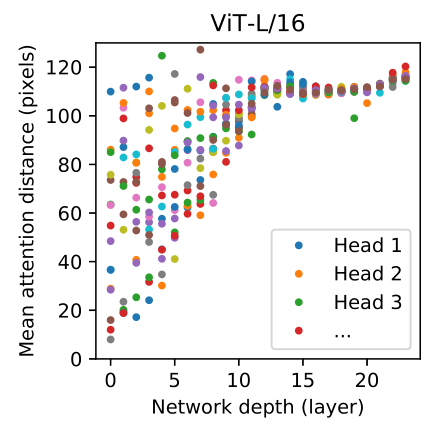
注意这里我们只使用了 attention，而没有使用 CNN，所以这里的 attention distance 相当于 CNN 的 receptive field 的大小。作者发现：在最底层，有些 head 也已经注意到了图像的大部分，说明模型已经可以 globally 地整合信息了，说明它们负责 global 信息的整合。其他的 head 只注意到图像的一小部分，说明它们负责 local 信息的整合。Attention Distance 随深度的增加而增加。

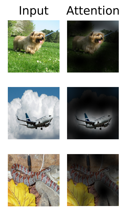
整合局部信息的 attention head 在混合模型 (有 CNN 存在) 时，效果并不好，说明它可能与 CNN 的底层卷积有着类似的功能。

作者给出了 attention 的可视化，注意到了适合分类的位置：

5.2 ViT 代码解读：

代码来自：

https://github.com/google-research/vision_transformer

首先是介绍使用方法：

安装：

pip install vit-pytorch

使用：

import torch
from vit_pytorch import ViT

v = ViT(
    image_size = 256,
    patch_size = 32,
    num_classes = 1000,
    dim = 1024,
    depth = 6,
    heads = 16,
    mlp_dim = 2048,
    dropout = 0.1,
    emb_dropout = 0.1
)

img = torch.randn(1, 3, 256, 256)
mask = torch.ones(1, 8, 8).bool() # optional mask, designating which patch to attend to

preds = v(img, mask = mask) # (1, 1000)

传入参数的意义：
image_size：输入图片大小。
patch_size：论文中 patch size： \(P\) 的大小。
num_classes：数据集类别数。
dim：Transformer 的隐变量的维度。
depth：Transformer 的 Encoder，Decoder 的 Layer 数。
heads：Multi-head Attention layer 的 head 数。
mlp_dim：MLP 层的 hidden dim。
dropout：Dropout rate。
emb_dropout：Embedding dropout rate。定义残差， \(\color{purple}{\text{Feed Forward Layer}}\) 等：

class Residual(nn.Module):
    def __init__(self, fn):
        super().__init__()
        self.fn = fn
    def forward(self, x, **kwargs):
        return self.fn(x, **kwargs) + x

class PreNorm(nn.Module):
    def __init__(self, dim, fn):
        super().__init__()
        self.norm = nn.LayerNorm(dim)
        self.fn = fn
    def forward(self, x, **kwargs):
        return self.fn(self.norm(x), **kwargs)

class FeedForward(nn.Module):
    def __init__(self, dim, hidden_dim, dropout = 0.):
        super().__init__()
        self.net = nn.Sequential(
            nn.Linear(dim, hidden_dim),
            nn.GELU(),
            nn.Dropout(dropout),
            nn.Linear(hidden_dim, dim),
            nn.Dropout(dropout)
        )
    def forward(self, x):
        return self.net(x)

Attention 和 Transformer，注释已标注在代码中：

class Attention(nn.Module):
    def __init__(self, dim, heads = 8, dim_head = 64, dropout = 0.):
        super().__init__()
        inner_dim = dim_head *  heads
        self.heads = heads
        self.scale = dim ** -0.5

        self.to_qkv = nn.Linear(dim, inner_dim * 3, bias = False)
        self.to_out = nn.Sequential(
            nn.Linear(inner_dim, dim),
            nn.Dropout(dropout)
        )

    def forward(self, x, mask = None):
# b, 65, 1024, heads = 8
        b, n, _, h = *x.shape, self.heads

# self.to_qkv(x): b, 65, 64*8*3
# qkv: b, 65, 64*8
        qkv = self.to_qkv(x).chunk(3, dim = -1)

# b, 65, 64, 8
        q, k, v = map(lambda t: rearrange(t, 'b n (h d) -> b h n d', h = h), qkv)

# dots:b, 65, 64, 64
        dots = torch.einsum('bhid,bhjd->bhij', q, k) * self.scale
        mask_value = -torch.finfo(dots.dtype).max

        if mask is not None:
            mask = F.pad(mask.flatten(1), (1, 0), value = True)
            assert mask.shape[-1] == dots.shape[-1], 'mask has incorrect dimensions'
            mask = mask[:, None, :] * mask[:, :, None]
            dots.masked_fill_(~mask, mask_value)
            del mask

# attn:b, 65, 64, 64
        attn = dots.softmax(dim=-1)

# 使用einsum表示矩阵乘法：
# out:b, 65, 64, 8
        out = torch.einsum('bhij,bhjd->bhid', attn, v)

# out:b, 64, 65*8
        out = rearrange(out, 'b h n d -> b n (h d)')

# out:b, 64, 1024
        out =  self.to_out(out)
        return out

class Transformer(nn.Module):
    def __init__(self, dim, depth, heads, dim_head, mlp_dim, dropout):
        super().__init__()
        self.layers = nn.ModuleList([])
        for _ in range(depth):
            self.layers.append(nn.ModuleList([
                Residual(PreNorm(dim, Attention(dim, heads = heads, dim_head = dim_head, dropout = dropout))),
                Residual(PreNorm(dim, FeedForward(dim, mlp_dim, dropout = dropout)))
            ]))
    def forward(self, x, mask = None):
        for attn, ff in self.layers:
            x = attn(x, mask = mask)
            x = ff(x)
        return x

ViT 整体：

class ViT(nn.Module):
    def __init__(self, *, image_size, patch_size, num_classes, dim, depth, heads, mlp_dim, pool = 'cls', channels = 3, dim_head = 64, dropout = 0., emb_dropout = 0.):
        super().__init__()
        assert image_size % patch_size == 0, 'Image dimensions must be divisible by the patch size.'
        num_patches = (image_size // patch_size) ** 2
        patch_dim = channels * patch_size ** 2
        assert num_patches > MIN_NUM_PATCHES, f'your number of patches ({num_patches}) is way too small for attention to be effective (at least 16). Try decreasing your patch size'
        assert pool in {'cls', 'mean'}, 'pool type must be either cls (cls token) or mean (mean pooling)'

        self.patch_size = patch_size

        self.pos_embedding = nn.Parameter(torch.randn(1, num_patches + 1, dim))
        self.patch_to_embedding = nn.Linear(patch_dim, dim)
        self.cls_token = nn.Parameter(torch.randn(1, 1, dim))
        self.dropout = nn.Dropout(emb_dropout)

        self.transformer = Transformer(dim, depth, heads, dim_head, mlp_dim, dropout)

        self.pool = pool
        self.to_latent = nn.Identity()

        self.mlp_head = nn.Sequential(
            nn.LayerNorm(dim),
            nn.Linear(dim, num_classes)
        )

    def forward(self, img, mask = None):
        p = self.patch_size

# 图片分块
        x = rearrange(img, 'b c (h p1) (w p2) -> b (h w) (p1 p2 c)', p1 = p, p2 = p)

# 降维(b,N,d)
        x = self.patch_to_embedding(x)
        b, n, _ = x.shape

# 多一个可学习的x_class，与输入concat在一起，一起输入Transformer的Encoder。(b,1,d)
        cls_tokens = repeat(self.cls_token, '() n d -> b n d', b = b)
        x = torch.cat((cls_tokens, x), dim=1)

# Positional Encoding：(b,N+1,d)
        x += self.pos_embedding[:, :(n + 1)]
        x = self.dropout(x)

# Transformer的输入维度x的shape是：(b,N+1,d)
        x = self.transformer(x, mask)

# (b,1,d)
        x = x.mean(dim = 1) if self.pool == 'mean' else x[:, 0]

        x = self.to_latent(x)
        return self.mlp_head(x)
# (b,1,num_class)